Introduction to Trino Cost-Based Optimizer

Last edited 15 June 2022: Update to use the Trino project name.

The Cost-Based Optimizer (CBO) in Trino achieves stunning results in industry standard benchmarks (and not only in benchmarks)! The CBO makes decisions based on several factors, including shape of the query, filters and table statistics. I would like to tell you more about what the table statistics are in Trino and what information can be derived from them.

This post was originally published at Starburst Data Engineering Blog.

Background #

Before diving deep into how Trino analyzes statistics, let’s set up a stage so that our considerations are framed in some context. Let’s consider a Data Scientist who wants to know which customers spend most dollars with the company, based on history of orders (probably to offer them some discounts). They would probably fire up a query like this:

SELECT c.custkey, sum(l.price)
FROM customer c, orders o, lineitem l
WHERE c.custkey = o.custkey AND l.orderkey = o.orderkey
GROUP BY c.custkey ORDER BY sum(l.price) DESC;

Now, Trino needs to create an execution plan for this query. It does so by first transforming a query to a plan in the simplest possible way — here it will create CROSS JOINS for FROM customer c, orders o, lineitem l part of the query and FILTER for WHERE c.custkey = o.custkey AND l.orderkey = o.orderkey. The initial plan is very naïve — CROSS JOINS will produce humongous amounts of intermediate data. There is no point in even trying to execute such a plan and Trino won’t do that. Instead, it applies transformation to make the plan more what user probably wanted, as shown below. Note: for succinctness, only part of the query plan is drawn, without aggregation (GROUP BY) and sorting (ORDER BY).

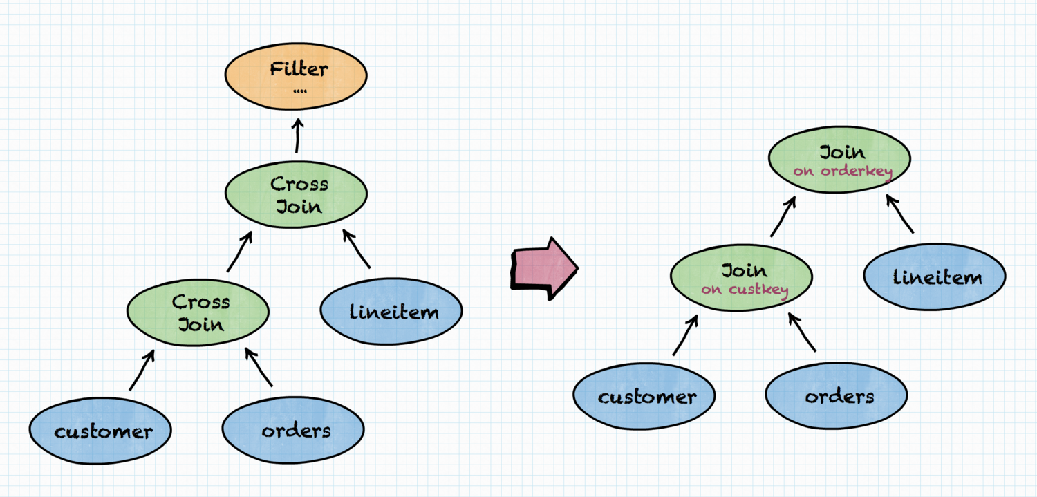
Indeed, this is much better than the CROSS JOINS. But we can do even better, if we consider cost.

Cost-Based Optimizer #

Without going into database internals on how JOIN is implemented, let’s take for granted that it makes a big difference which table is right and which is left in the JOIN. (Simple explanation would be that the table on the right basically needs to be kept in the memory while JOIN result is calculated). Because of that, the following plans produce same result, but may have different execution time or memory requirements.

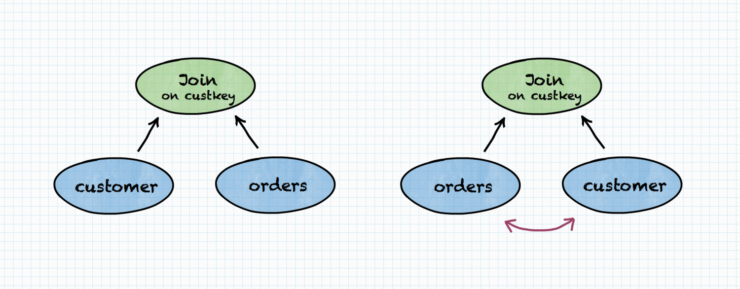
CPU time, memory requirements and network bandwidth usage are the three dimensions that contribute to query execution time, both in single query and concurrent workloads. These dimensions are captured as the cost in Trino.

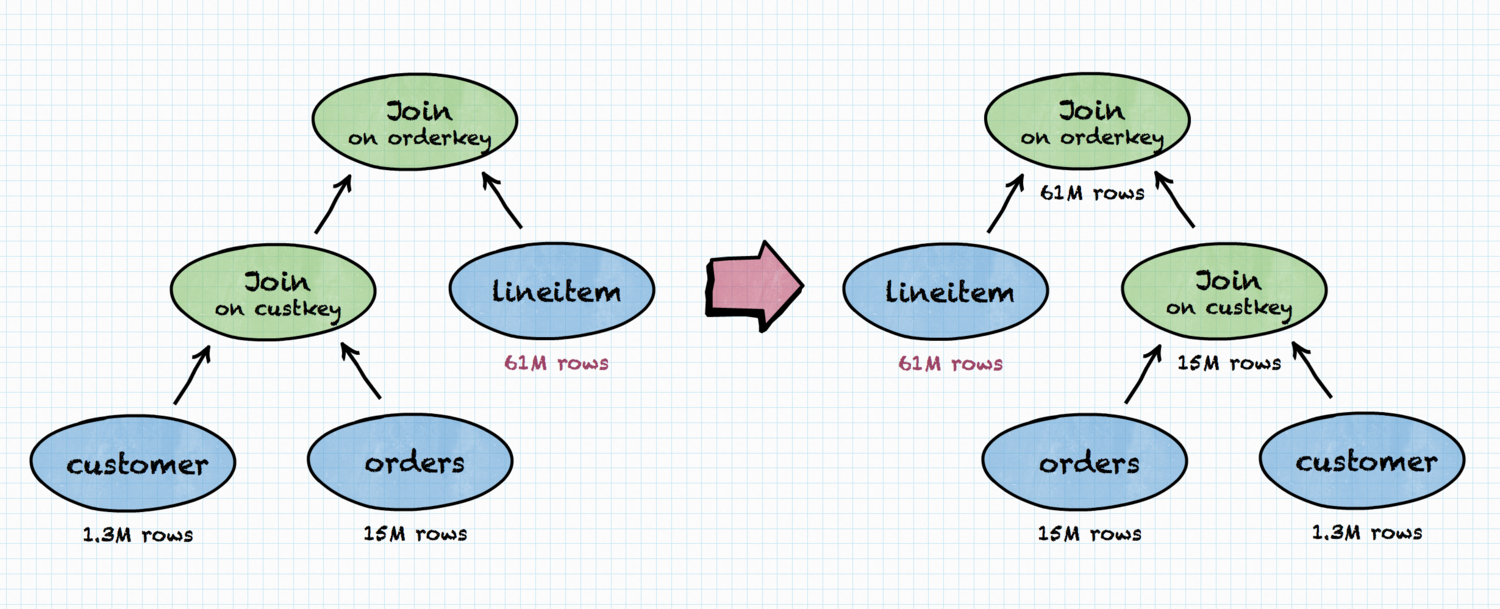
Our Data Scientist knows that most of the customers made at least one order and every order had at least one item (and many orders had many items), so lineitem is the biggest table, orders is medium and customer is the smallest. When joining customer and orders, having orders on the right side of the JOIN is not a good idea! However, how the planner can know that? In the real world, the query planner cannot reliably deduce information just from table names. This is where table statistics kick in.

Table statistics #

Trino has connector-based architecture. A connector can provide table and column statistics:

• number of rows in a table,
• number of distinct values in a column,
• fraction of NULL values in a column,
• minimum/maximum value in a column,
• average data size for a column.

Of course, if some information is missing — e.g. average text length in a varchar column is unknown — a connector can still provide other information and Cost-Based Optimizer will be able to use that.

In our Data Scientist’s example, data sizes can look something like the following:

Having this knowledge, Trino’s Cost-Based Optimizer will come up with completely different join ordering in the plan.

Filter statistics #

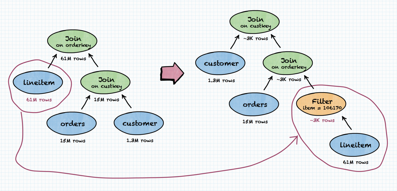
As we saw, knowing the sizes of the tables involved in a query is fundamental to properly reordering the joins in the query plan. However, knowing just the sizes is not enough. Returning to our example, the Data Scientist might want to drill down into results of their previous query, to know which customers repeatedly bought and spent most money on a particular item (clearly, this must be some consumable, or a mobile phone). For this, they will use almost identical query as the original one, adding one more condition.

SELECT c.custkey, sum(l.price)
FROM customer c, orders o, lineitem l
WHERE c.custkey = o.custkey AND l.orderkey = o.orderkey
  AND l.item = 106170                              --- additional condition
GROUP BY c.custkey ORDER BY sum(l.price) DESC;

The additional FILTER might be applied after the JOIN or before. Obviously, filtering as early as possible is the best strategy, but this also means the actual size of the data involved in the JOIN will be different now. In our Data Scientist’s example, the join order will indeed be different.

Under the Hood #

Execution Time and Cost #

From external perspective, only three things really matter:

• execution time,
• execution cost (in dollars),
• ability to run (sufficiently) many concurrent queries at a time.

The execution time is often called “wall time” to emphasize that we’re not really interested in “CPU time” or number of machines/nodes/threads involved. Our Data Scientist’s clock on the wall is the ultimate judge. It would be nice if they were not forced to get coffee/eat lunch during each query they run. On the other hand, a CFO will be interested in keeping cluster costs at the lowest possible level (without, of course, impeding employees’ effectiveness). Lastly, a System Administrator needs to ensure that all cluster users can work at the same time. That is, that the cluster can handle many queries at a time, yielding enough throughput that “wall time” observed by each of the users is satisfactory.

It is possible to optimize for only one of the above dimensions. For example, we can have single node cluster and CFO will be happy (but employees will go somewhere else). Contrarily, we may have thousand node cluster even if the company cannot afford that. Users will be (initially) happy, until the company goes bankrupt. Ultimately, however, we need to balance these trade-offs, which basically means that queries need to be executed as fast as possible, with as little resources as possible.

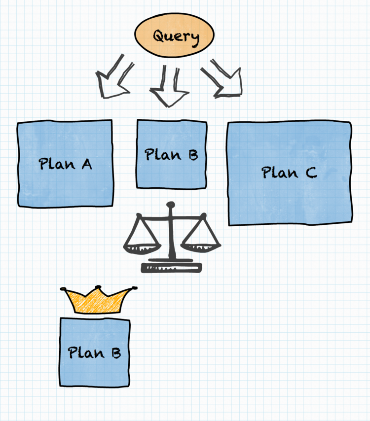
In Trino, this is modeled with the concept of the cost, which captures properties like CPU cost, memory requirements and network bandwidth usage. Different variants of a query execution plan are explored, assigned a cost and compared. The variant with the least overall cost is selected for execution. This approach neatly balances the needs of cluster users, administrators and the CFO.

The cost of each operation in the query plan is calculated in a way appropriate for the type of the operation, taking into account statistics of the data involved in the operation. Now, let’s see where the statistics come from.

Statistics #

In our Data Scientist’s example, the row counts for tables were taken directly from table statistics, i.e. provided by a connector. But where did “~3K rows” come from? Let’s dive into some nitty-gritty details.

A query execution plan is made of “building block” operations, including:

• table scans (reading the table; at runtime this is actually combined with a filter)
• filters (SQL’s WHERE clause or any other conditions deduced by the query planner)
• projections (i.e. computing output expressions)
• joins
• aggregations (in fact there are a few different “building blocks” for aggregations, but that’s a story for another time)
• sorting (SQL’s ORDER BY)
• limiting (SQL’s LIMIT)
• sorting and limiting combined (SQL’s ORDER BY .. LIMIT .. deserves specialized support)
• and a lot more!

The way how the statistics are computed for most interesting “building blocks” is discussed below.

Table Scan statistics #

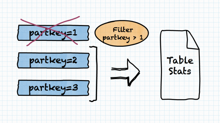
As explained in “Table statistics” section, the connector which defines the table is responsible for providing the table statistics. Furthermore, the connector will be informed about any filtering conditions that are to be applied to the data read from the table. This may be important e.g. in the case of Hive partitioned table, where statistics are stored on per-partition basis. If the filtering condition excludes some (or many) partitions, the statistics will consider smaller data set (remaining partitions) and will be more accurate.

To recall, a connector can provide the following table and column statistics:

• number of rows in a table,
• number of distinct values in a column,
• fraction of NULL values in a column,
• minimum/maximum value in a column,
• average data size for a column.

Filter statistics #

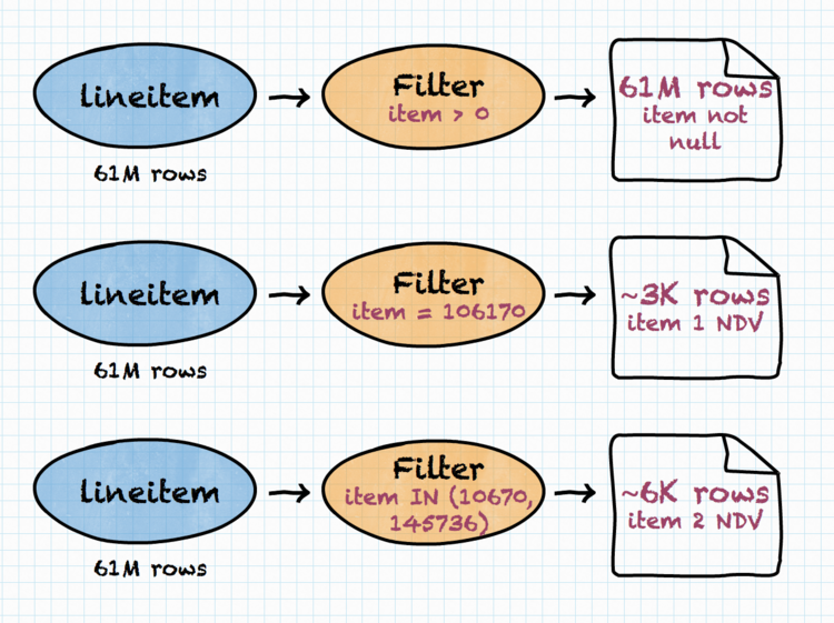
When considering a filtering operation, a filter’s condition is analyzed and the following estimations are calculated:

• what is the probability that data row will pass the filtering condition. From this, expected number of rows after the filter is derived,
• fraction of NULL values for columns involved in the filtering condition (for most conditions, this will simply be 0%),
• number of distinct values for columns involved in the filtering condition,
• number of distinct values for columns that were not part of the filtering condition, if their original number of distinct values was more than the expected number of data rows that pass the filter.

For example, for a condition like l.item = 106170 we can observe that:

• no rows with l.item being NULL will meet the condition,
• there will be only one distinct value of l.item (106170) after the filtering operation,
• on average, number of data rows expected to pass the filter will be equal to number_of_input_rows * fraction_of_non_nulls / distinct_values. (This assumes, of course, that users most often drill down in the data they really have, which is quite a reasonable assumption and also safe to make).

Projection statistics #

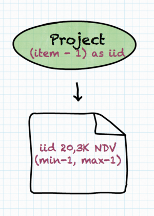
Projections (l.item – 1 AS iid) are similar to filters, except that, of course, they do not impact the expected number of rows after the operation.

For a projection, the following types of column statistics are calculated (if possible for given projection expression):

• number of distinct values produced by the projection,
• fraction of NULL values produced by the projection,
• minimum/maximum value produced by the projection.

Naturally, if iid is only returned to the user, then these statistics are not useful. However, if it’s later used in filter or join operation, these statistics are important to correctly estimate the number of rows that meet the filter condition or are returned from the join.

Conclusion #

Summing up, Trino’s Cost-Based Optimizer is conceptually a very simple thing. Alternative query plans are considered, the best plan is chosen and executed. Details are not so simple, though. Fortunately, to use Trino, one doesn’t need to know all these details. Of course, anyone with a technical inclination that like to wander in database internals is invited to study the Trino code!

Enabling Trino CBO is really simple:

• set optimizer.join-reordering-strategy=AUTOMATIC and join-distribution-type=AUTOMATIC in your config.properties,
• analyze your tables,
• no, there is no third step. That’s it!

Take Trino CBO for a spin today and let us know about your Trino experience!

□