Last month we called Trino 482 the summer of grammar release, because it closed so many small gaps in Trino’s dialect of SQL at once. Those additions were mostly about breadth: a long list of standard predicates and forms, each a modest convenience on its own.
Trino 483 keeps the season going, but the character is different. This release
lands a handful of larger, more powerful additions instead of a dozen small gaps.
They change the shape of the queries you write rather than just tidying them
up. One of them, PIVOT, is big enough to carry the release on its own. As
before, every example is live. Hit Run and watch Trino 483 evaluate it.
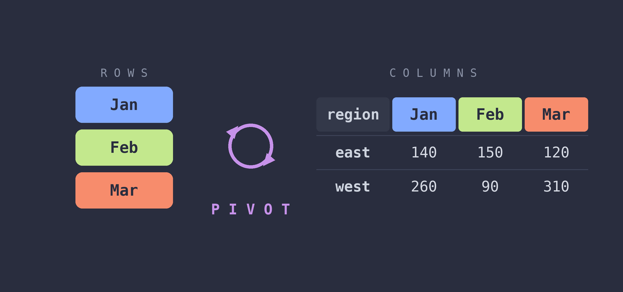
PIVOT, at last #
The headline feature is the PIVOT clause. If
you’ve ever written a pile of CASE expressions wrapped in aggregates to
turn a categorical column into a column per category, this is for you.
Every example in this section runs against the same little sales table: one row
per region, channel, and month, with an amount. To see why PIVOT is one of the
longest-standing feature requests, start with what you had to write before: one
sum(CASE ...) per month, spelled out by hand, with the column names left as
your own bookkeeping.
SELECT region,
       sum(CASE WHEN month = 1 THEN amount END) AS jan_total,
       sum(CASE WHEN month = 2 THEN amount END) AS feb_total
FROM (VALUES
    ('east', 'web',   1, 100),
    ('east', 'store', 1,  40),
    ('east', 'web',   2, 150),
    ('west', 'web',   1, 200),
    ('west', 'store', 1,  60),
    ('west', 'store', 2,  90)
) AS sales(region, channel, month, amount)
GROUP BY region
PIVOT says the same thing declaratively. You provide one or more aggregations,
a pivot column whose values become the new columns, and the list of values you
care about. Each additional month is just another entry in the IN list rather
than another hand-written CASE:
SELECT *
FROM (VALUES
    ('east', 'web',   1, 100),
    ('east', 'store', 1,  40),
    ('east', 'web',   2, 150),
    ('west', 'web',   1, 200),
    ('west', 'store', 1,  60),
    ('west', 'store', 2,  90)
) AS sales(region, channel, month, amount)
PIVOT (
    sum(amount) AS total
    FOR month IN (1 AS jan, 2 AS feb)
    GROUP BY region
)
The output has columns region, jan_total, and feb_total. Each pivoted
column name is stitched together from the pivot value’s alias and the
aggregation’s alias, and the GROUP BY names the dimensions that survive as
ordinary columns.
More than one number per cell #
A PIVOT can compute several aggregations at once. When it does, each one needs
an alias, so the pivot can build unambiguous column names by pairing every value
with every aggregation. In the following example each month gets both a total
amount and an order count:
SELECT *
FROM (VALUES
    ('east', 'web',   1, 100),
    ('east', 'store', 1,  40),
    ('east', 'web',   2, 150),
    ('west', 'web',   1, 200),
    ('west', 'store', 1,  60),
    ('west', 'store', 2,  90)
) AS sales(region, channel, month, amount)
PIVOT (
    sum(amount) AS total,
    count(*) AS orders
    FOR month IN (1 AS jan, 2 AS feb)
    GROUP BY region
)
The result gains jan_total, jan_orders, feb_total, and feb_orders: the
columns for each value stay grouped together, in the order the aggregations are
declared. The aggregation slot is a full expression, not just a bare function
call, so sum(amount) - sum(refund) AS net or
sum(amount) FILTER (WHERE amount > 0) AS gains are equally valid, and the pivot
value scoping applies to every aggregate inside the slot.
Subtotals with grouping sets #
Want a bottom-line total across all regions, and not just a row per region? You
don’t have to run a second query and staple it on. The GROUP BY inside a
PIVOT accepts the same forms as a top-level one, so GROUPING SETS, CUBE, and
ROLLUP come along for free. Wrapping region in a ROLLUP adds a grand-total
row, with region left NULL:
SELECT *
FROM (VALUES
    ('east', 'web',   1, 100),
    ('east', 'store', 1,  40),
    ('east', 'web',   2, 150),
    ('west', 'web',   1, 200),
    ('west', 'store', 1,  60),
    ('west', 'store', 2,  90)
) AS sales(region, channel, month, amount)
PIVOT (
    sum(amount) AS total
    FOR month IN (1 AS jan, 2 AS feb)
    GROUP BY ROLLUP (region)
)
Pivoting on more than one dimension #
The pivot column can be a tuple. Name a parenthesized list of columns in the
FOR clause and supply matching tuples in the IN list, and each combination
becomes its own column. This is how you build a cell per (channel, month) pair:
SELECT *
FROM (VALUES
    ('east', 'web',   1, 100),
    ('east', 'store', 1,  40),
    ('east', 'web',   2, 150),
    ('west', 'web',   1, 200),
    ('west', 'store', 1,  60),
    ('west', 'store', 2,  90)
) AS sales(region, channel, month, amount)
PIVOT (
    sum(amount) AS total
    FOR (channel, month) IN (
        ('web', 1) AS web_jan,
        ('web', 2) AS web_feb,
        ('store', 1) AS store_jan
    )
    GROUP BY region
)
Notice west’s web_feb_total comes back NULL: no row matches that
combination, so the aggregate sees an empty input. That is the one sharp edge to
remember. The IN list is a fixed set of constants you write out, so PIVOT
only produces columns for the values you name, and a value that never appears in
the data still produces a column full of empty-input results.
Because the result of a PIVOT is itself just a relation, it can be aliased,
nested in a subquery, or fed straight into another PIVOT.
Navigating JSON without the ceremony #
Trino has always had powerful tools for querying JSON, such as json_query,
json_value, and json_exists, but they
ask you to write out a full JSON path expression and a RETURNING clause for
even the simplest lookup. The SQL specification also defines a more convenient
simplified accessor syntax. Trino 483
now implements it and lets you reach into a json value with the same dotted
and subscripted notation you’d use on a row or an array.
The receiver has to be a value of the json type. Below, a JSON literal
supplies the document. Watch out for one trap: CAST('...' AS json) does not
parse the text into an object. It wraps the whole string as a single JSON string
value, and the accessor then quietly hands you back NULL. Use a JSON literal,
as shown here, to get an actual document. From there, each .member, [index],
or .method() step extends the path for you:
SELECT j.name.string() AS name,
       j.items[0].price.decimal(10,2) AS first_item_price
FROM (VALUES JSON '{"name": "Ada", "items": [{"price": 9.99}, {"price": 19.99}]}') t(j)
The trailing .string() on j.name is an item method that plays the role of
the old RETURNING varchar clause, and j.items[0].price.decimal(10,2) shows a
subscript and nested members composing in a single chain. There’s an item method
for every type json_value can return (.bigint(), .date(), .decimal(p, s),
.timestamp(), and so on), so the whole extraction reads fluently.
One thing worth internalizing: member names are matched case-sensitively
against the JSON keys, because the JSON path language is case-sensitive. So
j.Foo and j.foo are different paths, unlike ordinary SQL identifiers. The
item-method names, on the other hand, are regular SQL identifiers and stay
case-insensitive.
There’s also a wildcard form. SELECT j.* expands to the top-level members of a
JSON object, returned as a single column holding a JSON array:
SELECT j.* AS (members)
FROM (VALUES JSON '{"a": 1, "b": 2, "c": 3}') t(j)
Parsing dates inside JSON paths #
Staying with JSON for a moment: SQL/JSON path expressions gained a datetime()
method, which parses a textual item into a proper date or time value from inside
the path itself. It takes an optional format template, so you can handle the
non-ISO date strings that turn up in real-world documents without post-processing
in SQL:
SELECT json_value('{"order_date": "17-07-2026"}',
                  'lax $.order_date.datetime("DD-MM-YYYY")'
                  RETURNING date) AS order_date
Without a format template, datetime() reads the value as the most specific of
date, time, or timestamp with or without a time zone that its shape
allows.
Do these two periods overlap? #
Anyone who has written the predicate for “do two date ranges intersect” knows
it’s easy to get subtly wrong. The boundary conditions are fiddly, and the
naive start1 <= end2 AND start2 <= end1 doesn’t say much about intent. The
standard OVERLAPS predicate now
expresses it directly. Each operand is a (start, end) pair, and the result is
true when the two periods share any instant:
SELECT (DATE '2026-06-01', DATE '2026-08-31')
           OVERLAPS (DATE '2026-08-01', DATE '2026-09-30') AS summer_meets_fall,
       (DATE '2026-01-01', DATE '2026-03-31')
           OVERLAPS (DATE '2026-06-01', DATE '2026-08-31') AS q1_meets_summer
The second element of a pair can also be an interval instead of an end point,
in which case the end is computed as start + interval, handy when you know a
period by its length rather than its endpoints. OVERLAPS uses half-open
semantics, so two periods that merely touch at a boundary don’t count as
overlapping. And since no corner of SQL escapes the question of null, a null
endpoint isn’t an error: it simply leaves that side of the period open-ended.
Geometry grows a third dimension #
The language additions have plenty of company. Trino 483 substantially expands the geospatial function library, and two themes stand out.
The first is real support for three-dimensional geometry. ST_Point now has
overloads that take a Z coordinate (and an SRID), there’s an ST_Z accessor to
read it back, and ST_Force2D / ST_Force3D let you add or drop the third
dimension at will. Crucially, Z coordinates and SRID metadata are now preserved
across serialization, format conversions, and the geometry operations that
should carry them through:
SELECT ST_Z(ST_Point(1, 2, DOUBLE '3')) AS z_coordinate
The second is reprojection. ST_Transform (and ST_TransformXY, which
leaves Z untouched) converts a geometry between coordinate reference systems by
EPSG SRID, so you can move between, say, WGS 84 longitude/latitude and Web
Mercator. Paired with the new ST_GeomFromEWKT, which parses well-known text
with an SRID= prefix, projecting a point takes one expression:
SELECT ST_AsText(
    ST_Transform(
        ST_GeomFromEWKT('SRID=4326;POINT (-71.0882 42.3607)'),
        3857)) AS web_mercator
Beyond those, there’s a whole batch of new constructors and operations:
ST_MakeLine, ST_Collect, ST_Polygonize, ST_VoronoiPolygons,
ST_MinimumBoundingCircle, ST_OrientedEnvelope, and the
geometry_collect_agg aggregate, among others. Here’s a line assembled from a
handful of points:
SELECT ST_AsText(
    ST_MakeLine(ARRAY[ST_Point(0, 0), ST_Point(1, 1), ST_Point(2, 0)])) AS line
A small one to finish #
Not every addition needs to reshape your queries. There’s a new
title_case function that capitalizes
the first letter of each word and lowercases the rest, the obvious companion to
the upper and lower you already know:
SELECT title_case('the trino summer of grammar') AS titled
Wrapping up #
Where 482 was about filling in the many small corners of standard SQL, 483 is about a few genuinely new capabilities:
- pivoting rows into columns,
- navigating JSON as if it were native, and
- asking a straightforward question about overlapping time.
Different flavor, same goal: a dialect of SQL that lets you say what you mean with less ceremony.
And that’s just the language side of the ledger. Trino 483 also ships char
column filter fixes, a redesigned Web UI now serving as the default, and a long
list of connector improvements across Delta Lake, Iceberg, Hive, and more.
Thirsty for the rest? The Trino 483 release
notes have the full accounting.
Happy querying!