9: Distributed hash-joins, and how to migrate to Trino

Audio

Video

Video sections

Release 351

Release Notes discussed: https://trino.io/docs/current/release/release-351.html

This release was really all about renaming everything from a client perspective to use Trino instead of Presto. Manfred will cover all the work that was done to do this for the release

Question of the week: How do I migrate from presto releases earlier than 350 to Trino releases 351?

https://trino.io/blog/2021/01/04/migrating-from-prestosql-to-trino.html

Concept of the week: Distributed Hash-join

Joins are one of the most useful and powerful operations performed by databases. There are many approaches to joining data. Various types of indices can facilitate joins. The order in which a join gets executed can vary depending on geographic distribution of the data, selectivity of the query where the fewer rows that get returned from a query the higher the selectivity, and the information available from indexes and table statistics can inform an execution engine how to form a query. One thing that stays consistent about virtually every query engine in the world is that they occur over two tables at a time no matter how many tables exist in the query. Some joins may occur in parallel but any given join will only involve two tables.

If you wrote a simple program that did what a join does, it might look something like a nested loop:

public class CartesianProductNestedLoop {
    public static void main(String[] args) {
        int[] outerTable = {2, 4, 6, 8, 10, 12};
        int[] innerTable = {1, 2, 3, 4};

        for (int o : outerTable) {
            for (int i : innerTable) {
                System.out.println(o + ", " + i);
            }
        }
    }
}

Since there is no predicate such as something you would see in a WHERE clause, the join returns the cartesian product of these two tables. It is useful also to portray these joins in relation algbegra. For example, the join above is written as $O \times I$ where $O$ is the outer table and $I$ is the inner table. $\times$ indicates that the join we are using is the cartesian product as we see below. Another useful way to view this is to visualize the join as a graph.

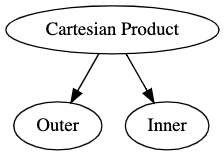
NOTE: When using relational algebra or using a graph to represent a join, it is convention that the table in the outer loop of this join is always shown on the left. This distinction becomes important as you will see below.

Here is the output from the cartesian product join above.

Notice also that we are treating these tables the same since we have to read each of the values to print out the cartesian product it doesn’t make a difference which table is the inner table and which is the outer yet. We could swap these tables for inner and outer and still get the same performance of $O (n^2)$.

Now, what if you did have some criteria that filtered out some rows that get returned from this product. Since it is quite common to join tables by an id, the most common criteria for a join is that the values are equal since values in rows with matching ids are related. Initially we can get away with just adding an if statement, print when true, and be done with it. Let’s do that.

public class NaturalJoinNestedLoop {
    public static void main(String[] args) {
        int[] outerTable = {2, 4, 6, 8, 10, 12};
        int[] innerTable = {1, 2, 3, 4};

        for (int o : outerTable) {
            for (int i : innerTable) {
                if(o == i){
                    System.out.println(o + ", " + i);
                }
            }
        }
    }
}

Lets assume that the integers in these tables are values of a column called id in both tables that uniquely identify a row in each table. When you have a commonly named column like this, the operation of joining based on columns that share the same name is a natural join. In relational algebra it is denoted with a litte bowtie, for example, $O \bowtie I$. We could also use the Equi-join notation that specifies the exact join columns $O \bowtie_(O.id = I.id) I$. The graph will look about the same as before but we only change the operation we are performing.

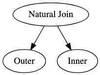
Now we only get the output of two rows as we should expect.

2, 2
4, 4

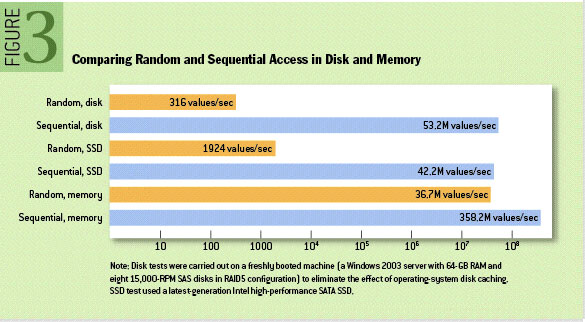
One important aspect that that gets glossed over in this simple example is that the data is small and in memory versus a database initially has to retrieve the data from disk. Reading values from a disk using random access is 100,000 times faster on memory. That being said, it’s really important to consider the fact that reading the values over and over again is going to be an exponential exercise, multiplied by 100,000.

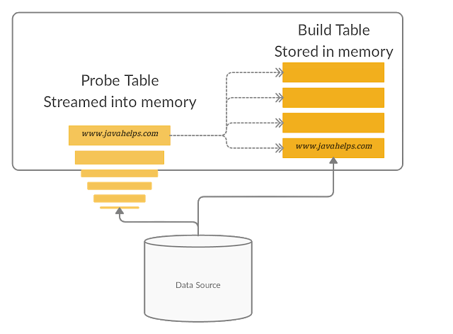
It would be better if we could read one table into memory once, and reuse those values as you scan over the data of the other table. There is a common name for both of these. Trino first reads the inner table into memory, to avoid having to read this table for each row in the outer table. We call this table the build table, as with the first scan you build the table in memory. Trino then streams the rows from the outer table and performs the join with the build table. We call this table the probe table.

import java.util.*;

public class BuildProbeLoops {
    public static void main(String[] args) {
        int[] probeTable = {2, 4, 6, 8, 10, 12};
        int[] buildTable = {1, 2, 3, 4};
        Map<Integer, Integer> buildTableCache = new HashMap<>();

        for (int row : buildTable) {
            //in this case the row is actually just the join column
            int hash = row;

            buildTableCache.put(hash, row);
        }

        for (int row : probeTable) {
            //in this case the row is actually just the join column
            int hash = row;

            Integer buildRow = buildTableCache.get(hash);
            if(buildRow != null){
                System.out.println(buildRow + ", " + row);
            }
        }
    }
}

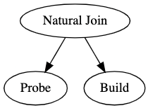
While it may seem redundant to do all of this extra work for this simple example, this saves minutes to hours when reading from disk and the data you are reading is big enough. The runtime complexity has now dropped from $O(n^2)$ to just a linear runtime of $O(n)$. The relational algebra for this table is now $P \bowtie B$, where $P$ is the probe table and $B$ is the build table. Notice the relational algebra for this hasn’t changed, we just now specify that we do a build on the inner table and probe the outer table.

One thing to consider is the size of each table, if we are fitting one of the tables into memory, it’s probably best we choose the smaller table to use as the build table. Hopefully this helps you understand now why we now specify between a build and a probe table. This will help in our discussions about query optimization and dynamic filtering which we will discuss on the next show.

Another interesting subtopic of this that we won’t get into today are left -deep and right-deep plans. Since now we know that the probe table is always on the left and our build table is on the right, the shape of our query matters. Consider the difference between these two trees.

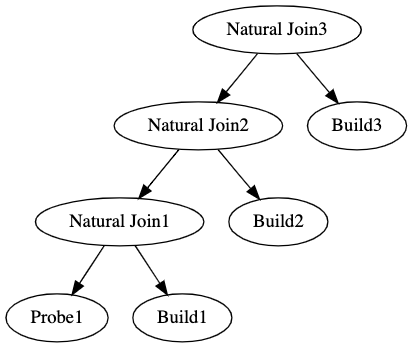
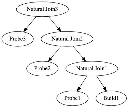
The left-deep tree vs right-deep trees have big implications on the speed of the query. This is a bit tangential for our talk today. Let’s finally move on to hash-joins!

In Trino, a hash-join is the common algorithm that is used to join tables. In fact the last snippet of code is really all that is invovled in implementing a hash-join. So in explaining probe and build, we have already covered how the algorithm works conceptually.

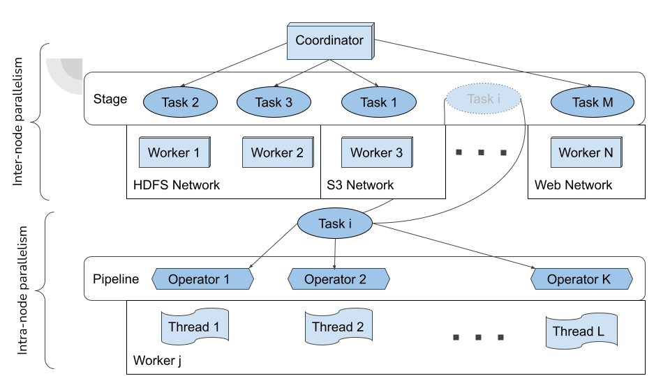
The big difference is that trino implements a distributed hash-join over two types of parallelism.

Joined tables are distributed over the worker nodes to achieve inter-node parallelism. Instead of the hash value simply being used to match with other rows, it is also used to route to specific Trino worker nodes. Rows that meet the equijoin criteria then are processed by the workers for a set of ids.
Within the node, workers can use the hash to further distribute the rows across multithreaded applications. This intranode-parallelism allows for there to be a single thread for every hash partition.
Finally, once all of these threads are finished determining which rows pass the join criteria, the probe side then begins to emit rows in larger batches, which can quickly be thrown out or kept based on which partitions exist on a given worker.

Great resources on this topic where some of the examples above derive:

How to contribute documentation and testimonials

Instead of a PR this week Manfred discusses some notes on how to contribute to documentation and testimonials.

If you want to show us some 💕, please give us a ⭐ on Github.

Events, news, and various links

Blogs

Upcoming events

Feb 9 - Feb 10 http://starburstdata.com/datanova

Latest training from David, Dain, and Martin(Now with timestamps!):

Presto® Summit Series - Real world usage

Podcasts:

If you want to learn more about Trino, check out the definitive guide from OReilly. You can download the free PDF or buy the book online.

Music for the show is from the Megaman 6 Game Play album by Krzysztof Słowikowski.

Do you ❤️ Trino? Give us a 🌟 on GitHub

Trino Community Broadcast